The first few decades of the 20th century sparked a revolution surrounding extremely small objects. Quantum mechanics upended the classical models of physics as they applied to particles at the atomic and subatomic level. Instead of being a smooth, continuous distribution, energy was actually quantized – there was a minimum amount of energy greater than zero, and energy increased by set increments.
The Bohr Model of the Atom #
Under classical principles, it was expected that an electron’s angular momentum would cause it to spiral into the nucleus and cause atomic collapse. This clearly was not happening, or else atomic collapse would be happening everywhere all the time. In 1914, Niels Bohr proposed a non-classical model of the atom that used the principle of quantization. His idea was that electrons could only travel in orbits of fixed radius around the atomic nucleus. Each “Bohr orbit” had a radius \(r\) defined in terms of an integer multiple \(n\) :
\[r = \frac{\epsilon_0 h^2}{\pi m_e e^2}n^2\]where \(n\) is a varying integer multiple.
Constants:
- \(\epsilon_0\) is electric permeability (the ability of a material to support the formation of a magnetic field), \(1.256 \times 10^{-6} \text{ N} \text{ A}^{-2}\) for free space
- \(h\) is Planck’s constant, \(6.626 \times 10^{-34} \text{ m}^2 \text{ kg} \text{ s}^{-1}\)
- \(m_e\) is the mass of an electron, \(9.109 \times 10^{-31} \text{ kg}\)
- \(e\) is the electric charge of an electron, \(-1.602 \times 10^{19} \text{ C}\)
Using \(n = 1\) in this equation gives a radius of \(5.29 \times 10^{-11} \text{ m}\) , also known as the Bohr radius. This is the minimum distance that an electron can be from the nucleus in a hydrogen atom. Since this is greater than zero, we know that an electron cannot actually crash into the nucleus like classical models suggested.
Bohr’s model was eventually proven wrong – electrons do not travel in circular orbits – but he still left a lasting impact on our thinking. Bohr hypothesized that the different orbit radii had energy levels associated with them. The energy levels followed this equation:
\[E_n = -R_y (\frac{1}{n^2})\]where \(n\) is an integer value associated with an energy level.
Constants:
- \(R_y\) is the Rydberg unit of energy, \(2.18 \times 10^{-18} \text{ J}\)
Note the negative sign, which reflects the attractive force between the electron and nucleus.
There are a couple cases to consider with this equation:
- \(n = 1\) is known as the ground state. This reflects the lowest possible energy state for the hydrogen atom. \(n > 1\) are the excited states of the atom.
- \(n \rightarrow \infty\) causes the energy to approach zero (remember, the energy is normally negative, so this is really high energy!) This causes the electron to completely break off from the atom, also known as ionization.
This means that the potential energy of an electron not bound to an atom is zero. As the nucleus and electron come closer, the reaction is favorable or stabilizing, causing the energy to decrease.
We can use the previous equation to calculate the energy difference between two states:
\[\Delta E_n = -R_y (\frac{1}{n_1^2} - \frac{1}{n_2^2})\]where \(n_1\) and \(n_2\) are integer values associated with energy levels.
Constants:
- \(R_y\) is the Rydberg unit of energy, \(2.18 \times 10^{-18} \text{ J}\)
Note the negative sign, which reflects the attractive force between the electron and nucleus.
Schrödinger, Born, and Atomic Orbital Wavefunctions #
Scientists in the 1920s realized that matter displayed a wave-particle duality – that is, it had properties of both a wave and a particle. Erwin Schrödinger created an equation that accounted for this fact:
\[H\Psi = E\Psi\]where \(H\) is the Hamiltonian operator (a fancy second-degree differential equation) and \(\Psi\) is a wavefunction (an equation that mathematically describes a particle). \(E\) is the total energy of the electron.
That’s great and all, but what does \(\Psi\) mean in a real-world context? Max Born proposed that \(\Psi\) was related to the probability of finding an electron in an atom. He ended up proving that \(|\Psi|^2\) was the probability density (the likelihood of finding something at any point in a given region). This meant that you could use Schrödinger’s equation to determine where an electron was probably located.
Now, there are a few limitations on \(\Psi\) as a result of this:
- \(0 \leq \Psi \leq 1\) , because if not the probability \(\Psi^2\) doesn’t make any sense.
- \(\Psi\) must be single-valued for a point. Having two different probabilities for a point also makes no sense.
- \(\Psi\) must be a smooth and continuous function to satisfy the requirements of the second-order differential equation.
In practice, \(\Psi\) for a hydrogen atom is made up of two parts: a radial function \(R\) and an angular function (or spherical harmonic function) \(Y\) . It follows this equation:
\[\Psi_{n, l, m_m} (r, \theta, \phi) = R_{n, l}(r) \cdot Y_{l}^{m_l}(\theta, \phi)\]where \((r, \theta, \phi)\) is the set of spherical coordinates for the electron’s location relative to the proton and \((n, l, m_m)\) is the set of quantum numbers associated with the electron.
We’ll ignore the angular function for now and focus on the radial function, which generally takes the form:
\[R(r) = Np(r)e^{-kr}\]where \(r\) is the distance between the electron and the nucleus.
Constants:
- \(N\) is a positive constant
- \(k\) is a positive constant
- \(p(r)\) is a polynomial function of \(r\)
This shows us that for the hydrogen atom, the probability of finding an electron at a specific location is dependent solely on the distance from that point to the nucleus.
The two simplest radial wavefunctions for the hydrogen atom are:
\[R_{1s} = 2(\frac{Z}{a_{0}})^{\frac{3}{2}}e^{\frac{-Zr}{a_{0}}}\] \[R_{2s} = 2(\frac{Z}{2a_{0}})^{\frac{3}{2}}(1-\frac{Zr}{2a_{0}})e^{\frac{-Zr}{2a_{0}}}\]
where \(r\) is the distance between the electron and the nucleus.
Constants:
- \(Z\) is the nuclear charge (in this case, \(+1\) )
- \(a_0\) is the Bohr’s radius, \(0.529 \text{ Å}\)
These functions are equivalent to Bohr’s \(n = 1\) and \(n = 2\) , respectively.
Here’s a graph showing how the probability density of the 1s and 2s orbitals varies with distance:
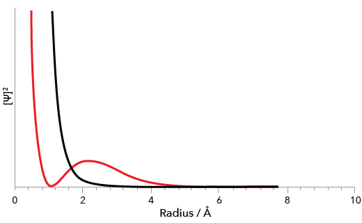
Probability density distribution of 1s and 2s orbitals of hydrogen.
The 1s orbital is the black curve, while the 2s orbital is plotted in red.
There’s a point around \(r = 0.6 \text{ Å}\) where the 2s probability density equals zero; that’s what’s called a node.